Snackwatch
Algorithm design and technical implementation
Introduction
Between 2019 and 2020, Justin, Joseph and I designed, prototyped, and validated Snackwatch, a fitness tracker that counts every bite of food you take. Snackwatch was set to be the flagship product for our health-wearables startup whose business model and product vision are detailed here. In summary we sought to improve diet journal accuracy to improve diet accountability and intervene in food addictive behaviors when indications such as fast eating or between-meal snacking presented. Though the technology worked phenomenally well achieving 93% accuracy in real world conditions and satisfactory subjective user ratings, we were forced to close our doors due to the emergence of patents on mission-critical, future features. This post details the technical development of the Snackwatch algorithm and prototype device.
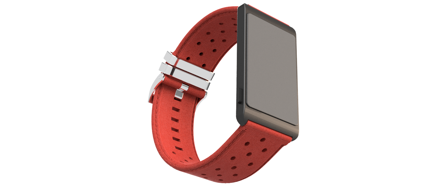
A render of Snackwatch as planned.
Project Scope
Having designed and launched wearable hardware before, our primary technical risk was whether or not we could produce an eating gesture classification model suitable for our application. Presently, binary classification of arbitrary gestures from inertial (accelerometer, gyroscope) data has only been solved in a few specific cases with limited accuracy. Without an off-the-shelf solution we had to develop our own with the following requirements:
- Any time a user wearing Snackwatch took a bite of food using a fork or spoon in the Snackwatch-wearing hand, the model must indicate a bite, and otherwise not indicate a bite.
- The model can only take a single stream of 3-axis accelerometer and gyroscope data as an input.
- The model must be efficient enough to run on an nRF52832 processor.
- The model must be trainable on a reasonably small data set, since we had to generate all our own training data.
Current State of Research
Inertial gesture classification is rather understudied since Bluetooth enabled inertial sensors were pretty unwieldy until relatively recently. The existing literature is sparse at best and somewhat low quality with most papers avoiding testing their models in free living environments. Regardless, there are three main approaches:
- Hidden Markov models
- Dynamic time warping
- Neural Nets
- Warping Longest Common Sub Sequence (WLCSS), an efficient version of the LCSS edit distance algorithm
After a review of the available research, we concluded that hidden Markov models and dynamic time warping were too power-intensive for our application and neural nets required far more training data than we could tolerate annotating ourselves. This left us with WLCSS, a rather new and obscure edit distance template-based algorithm developed by Roggen et al. WLCSS is specifically designed for low power pattern recognition and has achieved fairly good accuracy in similar gesture classification applications.
Methods
Data Collection
Your model is only as good as your data. To build up our data set, we sat ourselves, our family, our friends, and basically anyone else we could find in front of a laptop webcam while wearing a Snackwatch. Snackwatch inertial data was streamed over Bluetooth to the laptop and synced with the video.
We then manually annotated, frame by frame, the start and end points of each bite as defined by when the hand starts moving towards the mouth and when the hand stops moving away from the mouth, respectively. This process was made somewhat less painful by a suite of in-house tools we developed using ffmpeg. Due to the data-efficiency of the algorithm detailed below, we ultimately only needed 485 training examples extracted from 1 hour, 47 minutes of video
Model
Our model ultimately ended up significantly more complex than Roggen’s original WLCSS algorithm as we improved accuracy by adding layers of abstraction above and below the WLCSS layer proper.
Feature Engineering
We used conventional signal processing techniques to produce a more expressive incoming data stream. An accelerometer simultaneously measures the acceleration of the object to which it is attached and also the pull of earth’s gravity. As a result, if the sensor reads +9.8m/s^2 in the z direction, it is unclear whether the sensor is accelerating upwards at 2g, or if it has simply turned upside down. Since we have access to angular velocity using the gyroscope, we can use sensor fusion to split the gravitational acceleration from the true acceleration using a complementary filter. We also implemented a moving average filter on each sensor input, giving us a total of 6 raw features and 12 engineered features of type [float].
Quantization
WLCSS computes the similarity between an incoming time series and a training template time series by computing the number of frames they share in common, where a frame is defined as the data arriving at a single point in time. Unlike dynamic time warping, WLCSS requires that data be quantized, which makes all single-frame “edits” equal in the eyes of the loss function. To use an analogy, WLCSS measures the difference between “fish” and “dish” as 1, but we must first use clustering to map our frames (of type [float]) to the symbols f, i, s, h, and d. We experimented with several methods and found a random forest to be the most effective.
We mixed in a bit of a trick to embed semantic meaning into the clustering output classes. Unlike prior literature, our random forest did not simply quantize the feature space into arbitrary partitions. Rather, we positive (bite-containing) training time series segments into n subsegments and trained our random forest classifier to identify where in the segment a frame was likely to fall based on its features with classes 1, 2, … occurring in the beginning of the bite and classes ... , n-2, n-1, n occurring at the end of the bite . In this way, we could expect that an incoming data stream with classes that generally increase with respect to time to be fairly bite-like. I personally believe this innovation to have radically decreased the amount of data necessary to train our model.
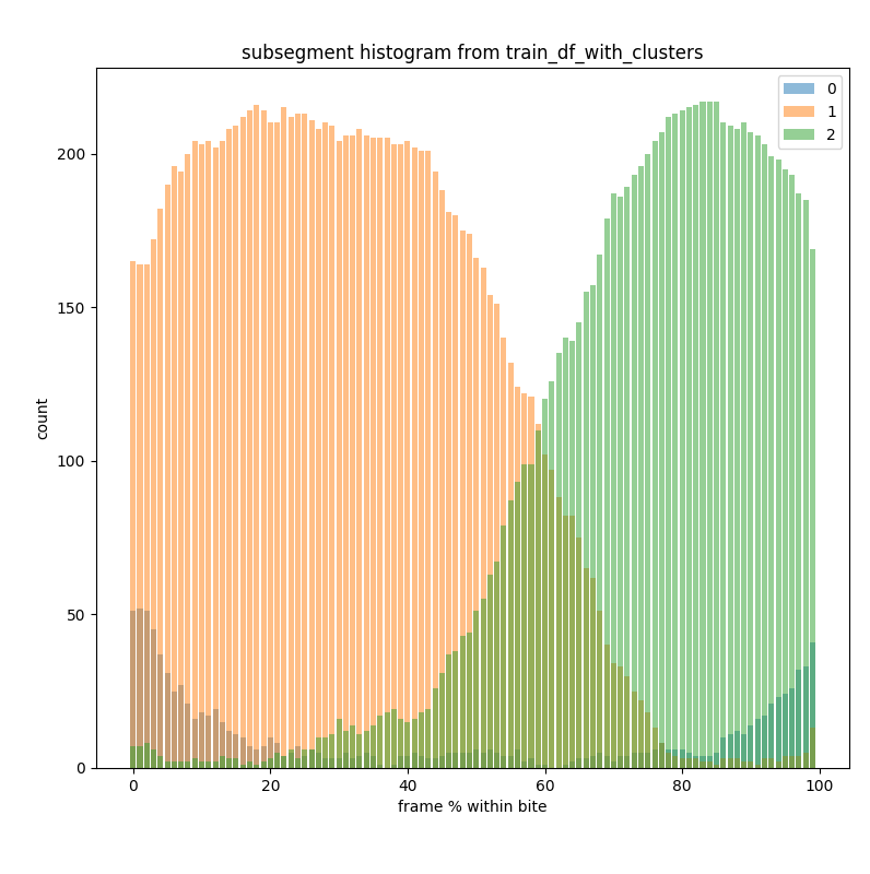
The distribution of frames classified as start of bite (1), end of bite (2), or not part of a bite (0). We see that class 1 frames largely appear in the first half of bites and class 2 frames largely appear in the second half of bites, for subsegments hyperparameter = 2. This suggests that the order of subsegment classes within a time series segment can be used to infer whether the segment is a bite (i.e. bites will look like 1,1,1,1,1,2,2,2,2.)
Template Selection
Now that we have quantized all our training data, we are able to select a set of k templates which we will use as the basis for what our model considers a bite. Incoming time series will be featurized and quantized and compared to all templates using WLCSS, with the minimum edit distance to any template being the returned value. While any set of templates could theoretically be used, the most generalizable set would be the one which best “spans” the training set by being most similar to all training examples. This problem is solved with the k-medoids algorithm.
Thresholding
Since running WLCSS between incoming data and our template set outputs an integer edit distance, we must select a threshold below which we classify incoming data as a bite and above which not a bite.
Hyperparameter Search
As you can see, this algorithm requires numerous hyperparameters, including the WLCSS threshold, the number of templates, the number of subsequences, the random forest parameters, and the moving average and complementary filter parameters. We implemented a Bayesian hyperparameter search for hyperparameter selection. Since our model is computed in layers, we also implemented a sophisticated in-house caching system called Hynet to entirely eliminate redundant computations. Hynet was effectively a disk-based memoization system that also accounted for function dependencies and code versions, permitting an order of magnitude speedup in training time. This infrastructure allowed us to train our model overnight on a single old laptop.
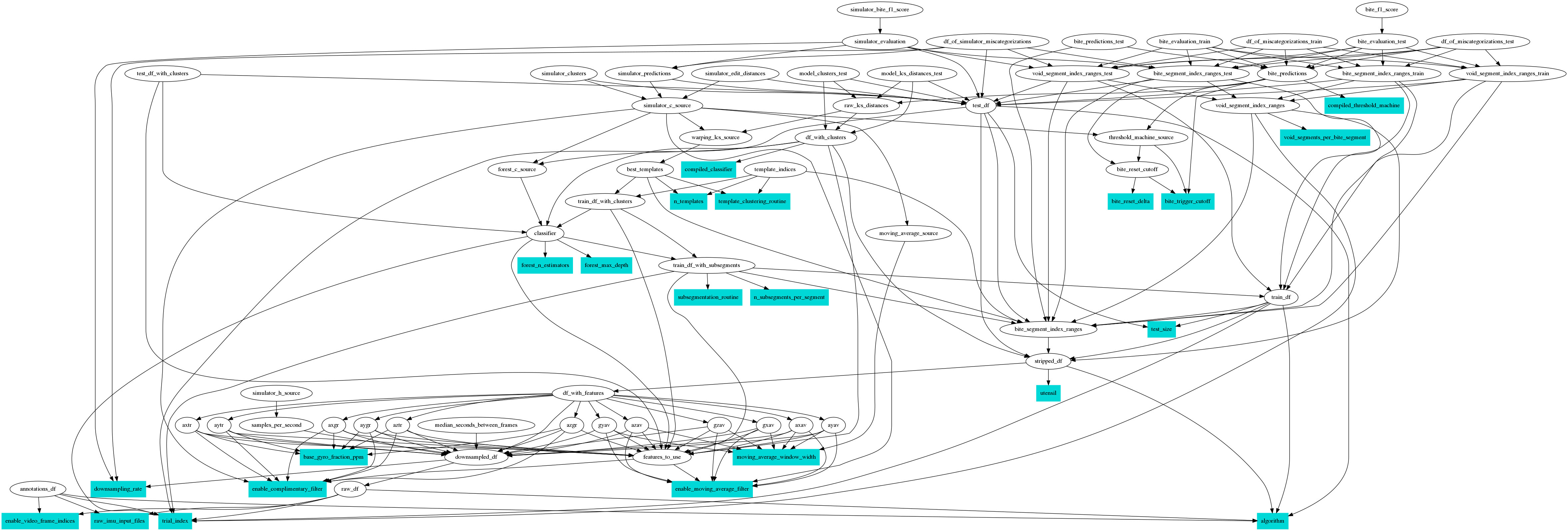
The dependency of functions within our model training algorithm with hyperparameters shown in blue. Since many functions are dependent on the results of other functions, it is important not to recompute the input functions for each new hyperparameter set being evaluated.
Simulator
In order to test our results in the real world, we reprogrammed our original collector laptop (see Data Collection) to simultaneously run the Snackwatch classification algorithm while it collects data. This allowed us to find false positives and false negatives in the model and immediately generate adversarial data to retrain the model.
Deployment
Once the simulator performed at an acceptable level, we rigged the data pipeline to output a c binary for deployment on our Snackwatch prototype.
Results
Our algorithm achieved an F1 accuracy of 90% with 96% recall and 84% precision. This level of accuracy is sufficient that were we to move forward with planned features like meal detection, it would be straightforward to detect clusters of bites to classify as meals. More importantly, our subjective accuracy was also very high. We equipped 8 volunteers with our simulator and had them eat either fried rice or a pastry using a fork. The Snackwatch simulator was configured to beep every time the subject took a bite. Of these volunteers, 7 of them described the accuracy as either very good or excellent.
Conclusion
Ultimately Snackwatch was a technical success on all fronts, achieving best-in-class results in real world scenarios. We were able to develop novel solutions to several unsolved problems including applying semantic analysis to WLCSS and applying caching to arbitrary functions in hyperparameter search. Our algorithm and data pipeline is architected in a strongly generalizable way meaning it could be repurposed to detect arbitrary complex gestures with little to no codebase changes. The toolchain and the algorithm itself may have application to other small data time series classification problems.